Tuto 6: Hybrid fermion-boson Hamiltonians: Hubbard-Holstein and polaritonic chemistry
Lucie Pepe - Laboratoire de Chimie Quantique de Strasbourg, France - January 2024
# Import libraries
import numpy as np
import scipy
import matplotlib.pyplot as plt
import quantnbody as qnb
In this second QuantNBody tutorial on hybrid models, we’ll show how to build two simple examples of hybrid systems composed of fermions and bosons interacting together.
Example 1: Hubbard-Holstein model
Fermionic Hubbard model:
In the local site basis, the Fermionic-Hubbard model Hamiltonian \(\hat{H}_{elec}\) is usually expressed such that:
with:
\(U_{iiii}\) the local coulombic repulsion on site “\(i\)”.
Adding the bosonic sub-part:
with \(\Omega_s\) the frequency of each mode \(s\), and \((\hat{b}^\dagger,\hat{b})\) the bosonic operators.
Adding the bosonic-fermionic interaction:
with \(\lambda_s\) the coupling of each mode \(s\) with the fermionic sub-system.
Step 1: Building the Hamiltonian
If we choose the following number of constituants:
# ======================================
# Define the fermionic system
# ======================================
N_elec_Holstein = 2 # number of fermions
N_MO_Holstein   = 2 # number of molecular orbitals

# ======================================
# Define the bosonic system
# ======================================
N_b_max_Holstein = 4 # maximal number of bosons in the whole bosonic system
N_mode_Holstein  = 2 # number of bosonic modes
list_bosons_Holstein = [ n for n in range(N_b_max_Holstein+1) ] # list of all possible number of bosons that can be distributed in the bosonic modes
One can directly use the implemented functions of the package to compute the associated nbody-basis of the hybrid system, as described previously:
# ==============================================
# Build the hybrid many-body basis and operators
# ==============================================
# Construct the basis
nbody_basis_Holstein = qnb.hybrid_fermionic_bosonic.tools.build_nbody_basis(N_mode_Holstein,
                                                                            list_bosons_Holstein,
                                                                            N_MO_Holstein,
                                                                            N_elec_Holstein)

# Build the fermionic particle conserving operator
a_dagger_a_Holstein = qnb.hybrid_fermionic_bosonic.tools.build_fermion_operator_a_dagger_a(nbody_basis_Holstein,
                                                                                           N_mode_Holstein)

# Build the bosonic creation (particle non-conserving) operator
b_Holstein = qnb.hybrid_fermionic_bosonic.tools.build_boson_anihilation_operator_b(nbody_basis_Holstein,
                                                                                   N_mode_Holstein)

# Build the bosonic annhilation operator : hermitian conjugate of the bosonic creation (particle non-conserving) operator
b_dag_Holstein = []
for mode in range(N_mode_Holstein):
    b_dag_Holstein += [b_Holstein[mode].T]
To obtain the whole Hamiltonian of the system, one has to use the obtained operators and the expression of the global Hamiltonian. Let’s first define all the parameters.
# ====================
# Define parameters
# ====================
t_val      = 1    # hopping term
U_val      = 10   # local coulombic repulsion
omega_val  = 10.0 # frequency, same for each mode
lambda_val = 1.0  # coupling of each mode with the fermionic sub-system
Coupling_fermion_boson = [lambda_val,lambda_val] # in a matrix form
The following step is the numerical computation of the one- and two-electron integrals of the fermionic-Hubbard part of the system.
# ======================
# Fermionic Hamiltonian
# ======================
t_  = np.zeros((N_MO_Holstein,N_MO_Holstein))
U_  = np.zeros((N_MO_Holstein,N_MO_Holstein,N_MO_Holstein,N_MO_Holstein))
for i in range(N_MO_Holstein):
    U_[i,i,i,i]  =  U_val  # Local coulombic repulsion
    for j in range(i+1,N_MO_Holstein):
        t_[i,j]  = t_[j,i] = - t_val  # Hopping constants

# ====================================
# Bosonic and interaction Hamiltonian
# ====================================
# Frequency of the modes in a matrix shape (here we have 2 modes)
omega_values = [omega_val, omega_val]
h_boson      = np.zeros((len(omega_values), len(omega_values)))
np.fill_diagonal(h_boson, omega_values)
Nevertheless, this model is already implemented in the package. One can just directly compute the whole Hamiltonian with the following line :
H_Holstein = qnb.hybrid_fermionic_bosonic.tools.build_hamiltonian_hubbard_holstein( t_,
                                                                                    U_,
                                                                                    a_dagger_a_Holstein,
                                                                                    h_boson,
                                                                                    b_Holstein,
                                                                                    Coupling_fermion_boson,
                                                                                    nbody_basis_Holstein)
Now we have the Hamiltonian, we can compute differentproperties of the systems. Let’s take a look at some examples of what can be done!
Step 2: Computing time-independent observables
Ground state values:
# Simply diagonalize the Hamiltonian
eig_energies_Holstein, eig_vectors_Holstein =  np.linalg.eigh(H_Holstein.A)
print('Energies =', eig_energies_Holstein[:4] )
Energies = [-0.58872733 -0.2 -0.2 -0.2 ]
We obtain here the groundstate energy and three subsequent degenerate excited states energies.
Occupation numbers:
# Compute the 2 bosonic occupation numbers in GS
occ_number_mode1 = eig_vectors_Holstein[:,0].T @ b_dag_Holstein[0] @ b_Holstein[0] @ eig_vectors_Holstein[:,0]
occ_number_mode2 = eig_vectors_Holstein[:,0].T @ b_dag_Holstein[1] @ b_Holstein[1] @ eig_vectors_Holstein[:,0]

print('Occ bosonic mode 1 =', occ_number_mode1 )
print('Occ bosonic mode 2 =', occ_number_mode2 )
Occ bosonic mode 1 = 0.01008950475957189
Occ bosonic mode 2 = 0.010089504759571898
Visualizing the GS WF in the many-body-basis:
WFT_GS = eig_vectors_Holstein[:,0]
WFT_visualize = qnb.hybrid_fermionic_bosonic.tools.visualize_wft(WFT_GS,
                                                                 nbody_basis_Holstein,
                                                                 N_mode_Holstein)
-----------
 Coeff.     N-body state and index
-------     ----------------------
-0.68715   |00⟩ ⊗ |1001⟩    #2
+0.68715   |00⟩ ⊗ |0110⟩    #3
-0.13356   |00⟩ ⊗ |0011⟩    #5
-0.13356   |00⟩ ⊗ |1100⟩    #0
+0.06871   |01⟩ ⊗ |1001⟩    #14
+0.06871   |10⟩ ⊗ |1001⟩    #8
-0.06871   |01⟩ ⊗ |0110⟩    #15
-0.06871   |10⟩ ⊗ |0110⟩    #9
+0.01995   |01⟩ ⊗ |0011⟩    #17
+0.01995   |10⟩ ⊗ |1100⟩    #6
-0.00683   |11⟩ ⊗ |1001⟩    #26
+0.00683   |11⟩ ⊗ |0110⟩    #27
+0.00676   |10⟩ ⊗ |0011⟩    #11
+0.00676   |01⟩ ⊗ |1100⟩    #12
Here we see that each state is decomposed as the tensor product of the bosonic part (2 modes here with a different number of bosonic occupancies, the maximum being 4 bosons) and a fermionic part (2 MOs here, so 4 digits for the 4 associated spinorbitals, with always 2 fermions since the number of fermionic particles remains unchanged).
Step 3: Computing time-dependent observables
Once all the components have been obtained, all the time-dependent observables can be easily calculated. We need to calculate the evolution operator for each time step and use it to compute the observables of interest at each instant. As an example, we’ll concentrate here on the occupancy number of each mode and fermionic molecular orbital.
# ====================
# Define parameters
# ====================
# Choose an initial state: a single hybrid configuration
many_body_state = [2,2,1,1,0,0] # Let's put 2 bosons in each mode, and the 2 electrons in the first MO orbital.

# Building the associated state in the qnb hybrid many-body basis
initial_state =  qnb.hybrid_fermionic_bosonic.tools.my_state( many_body_state,
                                                              nbody_basis_Holstein)

# Define time-dependent parameters
Nb_points = 1000
t_fin     = 1e2
list_t    = np.linspace( start=0, stop=t_fin, num=Nb_points )
# ==================================
# Compute time-dependent populations
# ==================================
pops_modes = np.zeros(( Nb_points, len(nbody_basis_Holstein[0])), dtype=float)
dim_H = len(nbody_basis_Holstein)
for time_index in range(Nb_points):

     # Building the evolution operator in the hybrid many-body basis
     U = np.zeros((dim_H,dim_H),dtype=np.complex128)
     for k  in range(dim_H):
         U +=  np.exp( -1j * eig_energies_Holstein[k] * list_t[time_index] ) * np.outer( eig_vectors_Holstein[:,k],  eig_vectors_Holstein[:,k].conj())

     # Determine the total wavefunction at each time step
     WF_T = U @ initial_state

     # Determine the occupation values in each site at each time-step
     for mode in range(len(nbody_basis_Holstein[0])):

        if mode  <= N_mode_Holstein -1 :
            # bosonic modes
            pops_modes[time_index,mode] += (( np.conjugate(WF_T).T) @( b_dag_Holstein[mode].A @ b_Holstein[mode].A) @ WF_T ).real
        else:
            # fermionic spin-orbitals
            pops_modes[time_index,mode] += (( np.conjugate(WF_T).T @ a_dagger_a_Holstein[mode- N_mode_Holstein,mode- N_mode_Holstein].A @ WF_T)).real
# ==================================
# Let's plot the results !
# ==================================

fig, (ax) = plt.subplots( nrows=2, ncols=1, figsize=(8, 6), sharex=(True) )

# Bosonic population of the 2 local bosonic modes
ax[0].plot( list_t, pops_modes[:,0]  ,  color='yellow', label='1st bosonic mode')
ax[0].plot( list_t, pops_modes[:,1] ,  color='black', label='2nd bosonic mode')
ax[0].set_xlim(0, 70)
ax[0].set_ylim(1.7, 2.1)
ax[0].grid(ls='--')
ax[0].legend(loc='upper right',fontsize='medium',  framealpha = 1 )
ax[0].set_ylabel('Populations', size=14)
ax[0].set_title('Population of bosonic modes', size=15)

# Fermionic populations of the two MOs
ax[1].plot( list_t, np.sum(pops_modes[:,2:], axis=1) ,  color='black', ls='dotted', label='total')
ax[1].plot( list_t, pops_modes[:,2] + pops_modes[:,3] ,  color='red', label='1st MO')
ax[1].plot( list_t, pops_modes[:,4] + pops_modes[:,5] ,  color='blue', label='2nd MO')

ax[1].set_xlim(0, 70)
ax[1].set_ylim(-0., 2.1)
ax[1].grid(ls='--')
ax[1].legend(loc='upper right', fontsize='medium',  framealpha = 1 )
ax[1].set_ylabel('Populations', size=14)
ax[1].set_xlabel('Time ($t^{-1}$ unit) ', size=14)
ax[1].set_title('Population of molecular orbitals', size=15)
fig.tight_layout()
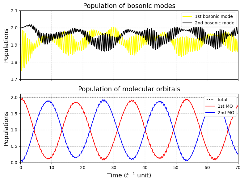
Example 2: Polaritonic chemistry
The QuantNBody package makes it possible to simulate polaritonic chemistry: an electronic structure system (model or ab-initio) in interaction with the photonic modes of a cavity. Here, as a proof of principle, we’ll concentrate on reproducing the FCI (Full Configuration Interaction) results obtained in the following article
U. Mordovina et al., Phys. Rev. Res., 2, 023262 (2020). For this reason, the molecular Hamiltonian here will be a fermi-Hubbard Hamiltonian.
Let’s first define the parameters of the total Hamiltonian of the system !
Electronic (Fermi-Hubbard) Hamiltonian:
With in the local site basis: -\(\hat{n}_{i,\sigma} = \hat{a}^\dagger_{i\sigma}\hat{a}_{i\sigma}\) the density of a spin-\(\sigma\) electron on site \(i\). -\(t_0\) and \(U\) the usual hopping and on-site repulsion constants. - The dipole operator of the system \(\hat{d} = \sum_i d_i ( \hat{n}_{i,\uparrow} + \hat{n}_{i,\downarrow} )\)
Cavity as a bosonic bath:
Here, \(\hat{b}_{\alpha}\) and \(\hat{b}^\dagger_{\alpha}\) represents the creation and annihilation operators for a cavity mode with frequency \(\omega_{c,\alpha}\).
Fermion-boson interaction:
Here, the coupling parameter \(\gamma_{\alpha}\) defines the strength of the light-matter interaction; here we focus mostly on the strong-coupling regime where \(\gamma_{\alpha}\) > 0.05. Note that in the following, every values will be expressed in \(t_0\) units (i.e., \(t_0 = 1\)).
Step 1: Building the Hamiltonian
As a proof-of-principle, we consider as in the reference paper U. Mordovina et al., Phys. Rev. Res., 2, 023262 (2020), a half-filled four site Hubbard chain with an additional dipole coupled to a single photon cavity mode with frequency \(\omega_{c,\alpha}= 1.028\). Here we consider \(\gamma = 0.2\) for the light-matter coupling parameter, representing an ultrastrong coupling.
# ======================================
# Define the fermionic system
# ======================================
N_elec_cavity = 4 # number of fermions
N_MO_cavity   = 4 # number of molecular orbitals

# ======================================
# Define the bosonic system
# ======================================
N_b_max_cavity = 7 # maximal number of bosons in the whole bosonic system
N_mode_cavity  = 1 # number of bosonic modes
list_bosons_cavity = [ n for n in range(N_b_max_cavity+1) ] # list of all the possible occupation number values that a bosonic mode can take

# ======================================
# Values of the parameters
# ======================================
U_val_cavity = 1     # on-site repulsion constant
t_val_cavity = 0.5   # hopping constant
gamma_cavity = 0.2   # coupling between bosons and fermions
freq_cavity  = 1.028 # cavity frequency
broad_cavity = 0.005 # broadening parameter for the GS absorption spectrum
Let’s now use the QuantNobdy functions to build the hybrid many-body basis, the operators, and finally the whole Hamiltonian of the system.
# ============================================================
# Build the hybrid many-body basis, operators and Hamiltonian
# ============================================================
# Construct the basis
nbody_basis_total_cavity  = qnb.hybrid_fermionic_bosonic.tools.build_nbody_basis(N_mode_cavity,
                                                                                 list_bosons_cavity,
                                                                                 N_MO_cavity,
                                                                                 N_elec_cavity )
dim_H_cavity = len(nbody_basis_total_cavity)

# Build the fermionic particle conserving operator
a_dagger_a_cavity  = qnb.hybrid_fermionic_bosonic.tools.build_fermion_operator_a_dagger_a(nbody_basis_total_cavity,
                                                                                          N_mode_cavity)

# Build the bosonic creation (particle non-conserving) operator
b_cavity  = qnb.hybrid_fermionic_bosonic.tools.build_boson_anihilation_operator_b(nbody_basis_total_cavity,
                                                                                  N_mode_cavity)

# Build the bosonic annhilation operator : hermitian conjugate of the bosonic creation operator
b_dag_cavity= []
for mode in range(N_mode_cavity):
    b_dag_cavity += [b_cavity[mode].T]

# Build the fermionic integrals
t_cavity       = np.zeros((N_MO_cavity,N_MO_cavity))
U_ferm_cavity  = np.zeros((N_MO_cavity,N_MO_cavity,N_MO_cavity,N_MO_cavity))
for i in range(N_MO_cavity):
    U_ferm_cavity[i,i,i,i]  =  U_val_cavity  # Local coulombic repulsion
    for j in range(N_MO_cavity):
        if j==i :
            t_cavity[i,j] = 0
        elif j==i+1 or j == i-1 :
            t_cavity[i,j] = t_cavity[j,i] = - t_val_cavity

# Building the dipole-related parameters
d_integrals = np.zeros((4,4), dtype = float)
d_integrals[0,0] = -1.5
d_integrals[1,1] = -0.5
d_integrals[2,2] = 0.5
d_integrals[3,3] = 1.5
d_integrals = np.array(d_integrals)

# Define them in a list for the implemented function of the QNB package
d_integrals_list    = np.diag(d_integrals)
cut_off_integral    = 1e-8
indices_d_integrals = np.transpose((abs(np.array(d_integrals))>cut_off_integral).nonzero())

# Build the dipole operator
d_op_cavity = scipy.sparse.csr_matrix((dim_H_cavity, dim_H_cavity))
for indices in indices_d_integrals:
    p = indices[0]
    d_op_cavity +=  d_integrals[p,p] * (a_dagger_a_cavity[2*p,2*p] + a_dagger_a_cavity[2*p+1,2*p+1])

# Build the total Hamiltonian
H_total_cavity  =  qnb.hybrid_fermionic_bosonic.tools.build_hamiltonian_hubbard_QED(t_cavity,
                                                                                    U_ferm_cavity,
                                                                                    a_dagger_a_cavity,
                                                                                    freq_cavity,
                                                                                    gamma_cavity,
                                                                                    d_integrals_list,
                                                                                    b_cavity,
                                                                                    nbody_basis_total_cavity)
Step 2: Computing time-independent properties
Let’s now use all the previously calculated ingredients to find the FCI values obtained in reference U. Mordovina et al., Phys. Rev. Res., 2, 023262 (2020).
Here, we focus on the case of a half-filled four-site Hubbard chain with an additional dipole coupled to a single photon cavity mode with frequency \(\omega_{c,\alpha}= 1.028\). We consider here \(\gamma= 0.2\) for the light-matter coupling parameter, representing ultra-strong coupling. For ultra-strong coupling, we have considered that the maximum number of bosons would be \(N_{B}^{max} = 7\). The values of the dipole in the site basis are taken here as \(d=[-1.5,-0.5, 0.5, 1.5]\). All these parameters are well defined in the legend of Table 1 (page 3) of U. Mordovina et al., Phys. Rev. Res., 2, 023262 (2020).
1) Ground state energies:
All the FCI ground energies are available in Table 1 (page 3) of the reference paper U. Mordovina et al., Phys. Rev. Res., 2, 023262 (2020), where different case of coupling (weak, strong, and ultrastrong) are indicated. Here, it has been shown that the FCI value of the ground state energy for the ultrastrong coupling (computed here as an example) is -1.41864. Let’s calculate this value with the QuantNBody package, by diagonalizing the Hamiltonian.
eig_energies_cavity, eig_vectors_cavity =  np.linalg.eigh(H_total_cavity.A)
print('Energies =', eig_energies_cavity[:4] )
Energies = [-1.41864225 -1.02867613 -1.02867613 -1.02867613]
Energies = [-1.41864225 -1.02867613 -1.02867613 -1.02867613]
Here we find the FCI value of the reference U. Mordovina et al., Phys. Rev. Res., 2, 023262 (2020). The ground state is followed by 3 degenerate excited states.
2) Occupation number of the bosonic mode in the ground state:
As for the ground state energies, All the FCI occupation numbers of the bosonic mode of the cavity are available in Table 1 (page 3) of the reference paper U. Mordovina et al., Phys. Rev. Res., 2, 023262 (2020), where different case of coupling (weak, strong, and ultrastrong) are indicated. Here, it has been shown that the FCI value of the bosonic mode occupation number for the ultrastrong coupling (computed here as an example) is 8.69 × 10⁻³. Let’s calculate this value with the QuantNBody package, using the computed \(\hat{b}\) and \(\hat{b}^\dagger\) operators :
occ_number_cavity = eig_vectors_cavity[:,0].T @ b_dag_cavity[0] @ b_cavity[0] @ eig_vectors_cavity[:,0]
print('occ_number : ', occ_number_cavity)
occ_number : 0.008692558807686325
Here we find again the FCI value of the FCI reference in U. Mordovina et al., Phys. Rev. Res., 2, 023262 (2020) with a great accuracy.
3) Ground-state absorption spectrum:
As defined in the Eq. 9 of the reference paper U. Mordovina et al., Phys. Rev. Res., 2, 023262 (2020) (page 3), the matter absorption cross section is given by :
where \(|\psi_k \rangle\) are many-body eigenstates of \(\hat{H}\) with energy \(\hbar \omega_k\) , \(\omega\) is the frequency of incident light, and \(\eta= 0.005\) is a (small) broadening parameter accounting for the finite lifetime of the state. Let’s compute the spectrum depicted in Fig 6.d of Appendix A (page 6) of the reference paper for the ultrastrong coupling case, using the parameters define in the related legend.
# Make the frequency vary
freq_spec_list = np.linspace(1e-6,4.5,700)
c = 1

# Calculate the cross section
cross_section = []
for freq_spec in freq_spec_list:
    somme = 0
    for k in range(dim_H_cavity)  :
        elem =  ((eig_vectors_cavity[:,k] @ d_op_cavity @ eig_vectors_cavity[:,0])**2.)   / ( (eig_energies_cavity[k] - eig_energies_cavity[0]) - freq_spec - 1j * broad_cavity  )
        somme += elem
    cross_section.append( 4* np.pi * ( freq_spec / c) * somme.imag)

# Plotting
fig, ( bx ) = plt.subplots( nrows=1, ncols=1, figsize=(6, 4), sharex=(True) )
bx.grid(linestyle='--')

bx.plot( freq_spec_list, np.log(cross_section) )
bx.set_ylabel('log $\\sigma$', size=14)
bx.set_xlabel('$\\omega$', size=14)
plt.tight_layout()
plt.show()
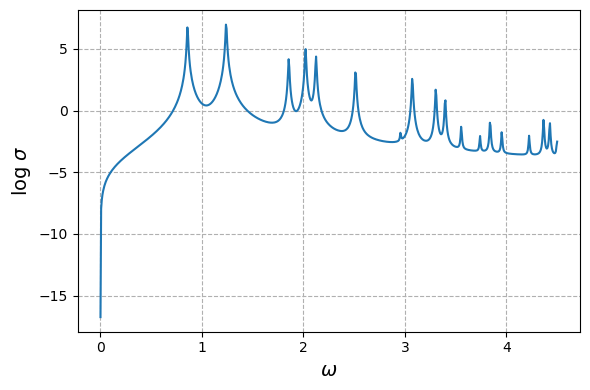
Here, we obtain the exact same spectrum than in the reference paper U. Mordovina et al., Phys. Rev. Res., 2, 023262 (2020).